Data formats
This chapter gives an overview of how image data is stored on a computer, and the challenges of storing and using huge 3D imaging data. It then uses these challenges to motivate and explain the development of the modern image storage formats, Zarr and OME-Zarr.
Storing data
All data in a computer is stored as binary, which is a series of 0s and 1s. One binary digit is called a bit. These are usually grouped together in batches of 8 bits, which together make a single byte.
A total of bits can represent any number in the range 0 to . So one byte (8 bits) can store any number from 0 to = 255, and two bytes (16 bits) can store any number from 0 to = 65,535.
Images are made up of a number of different pixels. In this book, for simplicity, we’ll focus on grayscale, or single-channel images. These are images where each pixel stores a single value. That’s a lot of words without a single image yet! Lets generate a random 16-bit 32 x 32 image as an example to take us through the rest of this chapter
import matplotlib.pyplot as plt
import numpy as np

image_shape = (32, 32)
dtype = np.uint16
image = np.random.randint(low=0, high=2**16, size=image_shape, dtype=dtype)
print(image)

fig, ax = plt.subplots()
ax.imshow(image, cmap="Grays", vmin=0, vmax=2**16);
Matplotlib is building the font cache; this may take a moment.
[[49092 15856 65490 ...  7087 23312  9710]
 [16944 44979 14071 ... 34960 29010 45141]
 [11876 58922 63671 ... 40737  2316 21997]
 ...
 [13453 16848 36808 ... 27866 17230  9609]
 [53541  3793 41063 ... 20590  4333 13620]
 [31658 44213 61353 ... 29751 57399  1459]]
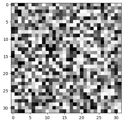
We can see what this looks like in binary, which is how the image is stored in memory:
image_bytes = image.tobytes()

print(f"{len(image_bytes)} bytes total")
print()
print("First ten bytes:")
for my_byte in image_bytes[:10]:
    print(f'{my_byte:0>8b}', end=' ')

print("...")
2048 bytes total
First ten bytes:
11000100 10111111 11110000 00111101 11010010 11111111 01111100 11111111 01110010 10000101 ...
Because we have an image with 1024 pixels, and each pixel is stored in 16 bits (2 bytes), we have a total of 10242 = 2048 bytes. Above you can see the bits written out for the first ten bytes of the image.
Saving images
So far the image we’ve worked on has been stored in the random access memory (RAM) on our computer. RAM is volatile, which means it’s erased when it loses power, so if we want to save our image or send it to someone else we have to save it to a file that lives on persistent storage (e.g., a hard drive).
There are lots of different file formats we can save 2D images to. The simplest way to save our image would be to save exact bits shown above to a file. To do this we can save our image to a TIFF file, a commonly used image file format in bio-sciences.
import imageio.v3 as iio

iio.imwrite("image_file.tiff", image, plugin='tifffile')
With no extra options specified, this saves the exact bits of the image to a file on disk. Because this TIFF file doesn’t compress the data, we should expect the file to be at least 2048 bytes big. Lets check:
import os.path

filesize_tiff = os.path.getsize("image_file.tiff")
print(f"File size: {filesize_tiff} bytes")
File size: 2304 bytes
The file is slightly bigger than 2048 bytes - the image itself takes up 2048 bytes and then other file metadata takes up some extra space.
Compression
This means the data stored in the TIFF file above is exactly the same as the data in memory. This makes the TIFF file very quick to read and write from, as the data doesn’t need to be processed or transformed at all, but just read directly into memory.
If we have limited storage space we might want to compress the data before writing it to a file to reduce the file size. In general there are two different types of compression:
- Lossless compression
- Lossy compression
A widely used example of a lossless image format is PNG:
iio.imwrite("image_file.png", image)
filesize_png = os.path.getsize("image_file.png")

print(f"TIFF file size: {filesize_tiff} bytes")
print(f"PNG  file size: {filesize_png} bytes")
TIFF file size: 2304 bytes
PNG file size: 2148 bytes
The PNG filesize is slightly smaller than the TIFF we saved with identical data. If we read the data back in from the PNG file, we still get exactly the same values back though:
image_png_data = iio.imread("image_file.png")
identical_png = np.all(image_png_data == image)
print(f"PNG: Recovered original data? {identical_png}")
PNG: Recovered original data? True
The cost of compressing the data is adding another step when reading or writing the data to file
Having to run compression (for saving the file) or decompression (for reading the file) slows down the time it takes to load or save an image.
If we want to compress the data further, we have to sacrifice some accuracy and use lossy compression. Lossy compression means that after saving and loading the data, the original data values are no longer recovered. A common example of a file format with lossy compression is JPEG. Here we’ll save to a JPEG2000 file, and check the file size and whether we recover the original image.
iio.imwrite("image_file.jp2", image, quality_layers=[2])
filesize_jpeg = os.path.getsize("image_file.jp2")

print(f"TIFF file size: {filesize_tiff} bytes")
print(f"PNG  file size: {filesize_png} bytes")
print(f"JPEG file size: {filesize_jpeg} bytes")
TIFF file size: 2304 bytes
PNG file size: 2148 bytes
JPEG file size: 1036 bytes
The JPEG file is much smaller than the others. But lets check if the data saved is the same as the original image data.
image_jp2_data = iio.imread("image_file.jp2")
identical_jpeg = np.all(image_jp2_data == image)
print(f"JPEG recovered original data? {identical_jpeg}")
JPEG recovered original data? False
We can see above that the original data isn’t recovered. To illustrate that further, the next plot shows the difference between the original data and the data stored in the JPEG file.
difference = image_jp2_data.astype(np.float32) - image.astype(np.float32)

fig, ax = plt.subplots()
im = ax.imshow(difference, cmap='RdBu')
fig.colorbar(im)
ax.set_title("Difference between original data and JPEG data");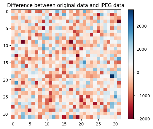
We’ve seen how to store 2D images, and the different compression options available. Introducing data compression can make reading and writing images slower, but reduces the filesize. Lossless compression saves the data without sacrificing any accuracy, and lossy compression results in even smaller file sizes but loses the original data values. In the next section we’ll explore how to store 3D images.
Storing large 3D data
One easy way of storing 3D data is to save it as a stack of 2D images. As an example, if we have an image with shape (10, 10, 20), we could save it to 20 2D image files, each of which has shape (10, 10). This is illustrated in the image below - each file is represented with a different colour.
Source
import matplotlib.figure

def color_chunk_figure(*, image_shape: tuple[int, int, int], chunk_shape: tuple[int, int, int]) -> matplotlib.figure.Figure:
    fig = plt.figure()
    ax = fig.add_subplot(projection='3d')

    for x in range(0, image_shape[0], chunk_shape[0]):
        for y in range(0, image_shape[1], chunk_shape[1]):
            for z in range(0, image_shape[2], chunk_shape[2]):
                voxels = np.zeros(image_shape)
                voxels[x:x+chunk_shape[0], y:y+chunk_shape[1], z:z+chunk_shape[2]] = 1
                ax.voxels(voxels, edgecolors='black', linewidths=0.5, alpha=0.9, shade=False);

    ax.set_aspect("equal")
    ax.axis('off');
    ax.set_title(f'Image shape = {image_shape}\nChunk shape = {chunk_shape}')
Source
color_chunk_figure(image_shape=(10, 10, 20), chunk_shape=(10, 10, 1))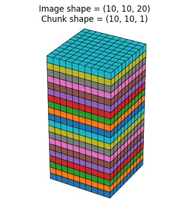
One way of thinking about this is that we are splitting the 3D image up into chunks, and each chunk is saved to a single file.
In this case each chunk has shape (nx, ny, 1), where nx and ny is the size of our 3D image in the x- and y- dimensions.
If we want to fetch a small cube of data from this 3D image, say shape (2, 2, 2), then we have to read and de-compress the two files that contain this data, and then we end up throwing away most of the data we’ve read in.
This is illustrated below - to get the data values at just 8 pixels (the red cubes), we have to read in 200 pixels in total (the orange cubes).
Source
fig = plt.figure()
ax = fig.add_subplot(projection='3d')

x, y, z = np.indices((10, 10, 20))

voxels = np.ones(x.shape)
voxels_request = (x < 4) & (x >= 2) & (y < 5) & (y >= 3) & (z < 4) & (z >= 2)
voxels_read = (z < 4) & (z >= 2)

all_vox = ax.voxels(voxels, alpha=0.2, edgecolors='black', linewidths=0.05, shade=False)
req_vox = ax.voxels(voxels_request, edgecolors='black', linewidths=0.5, facecolors='tab:red', alpha=1, shade=False);
read_vox = ax.voxels(voxels_read, edgecolors='black', linewidths=0.5, facecolors='tab:orange', alpha=0.3, shade=False);

ax.axis('off')
ax.set_aspect('equal')

custom_lines = [
    list(all_vox.values())[0],
    list(req_vox.values())[0],
    list(read_vox.values())[0]]
ax.legend(custom_lines, [
    'All data',
    f'Requested data ({np.sum(voxels_request)} voxels)',
    f'Read data ({np.sum(voxels_read)} voxels)'])
ax.set_title("Chunk shape = (10, 10, 1)")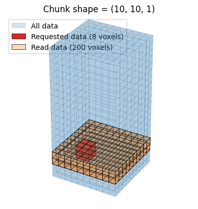
Compressing and saving 3D images as stacks of 2D images works well for small to medium sized 2D images, when reading each 2D image is fast, but what about large 3D data? As an example, one high resolution scan of a human heart from the Human Organ Atlas is 16 bit and has dimensions 7614 x 7614 x 8480. That’s 491,611,006,080 pixels (almost 500 billion), and 983 GB of data.
Add timings for reading in a large JPEG2000 image
As well as being slow to read, slices of large datasets are often much bigger than we actually want. As an example, I’m currently writing this text on a laptop with a screen resolution of 2560 x 1664. Even if I read in a full resolution 7164 x 7164 image, my computer can’t display all the pixels.
So for a better data format we want the following features:
- Less wasted effort when reading in small subsets of data
- Some way of storing low-resolution copies of the original image, for faster loading when zooomed out
These two requirements have spawned new data formats specifically designed to address these challenges. For the first challenge, we’ll look at how the Zarr format allows us to load load small subsets of data at a time. For the second challenge, we’ll look at how the OME-Zarr format extends Zarr to provide a way of storing multiple copies of the same image at different resolutions.
Zarr
In the example above where we stored 3D data as a series of 2D image files, the chunk shape of our data was (nx, ny, 1).
This means each file that makes up the full dataset contains a data array that has shape (nx, ny, 1).
If we want to read a single pixel, this is the minimum amount of data we need to load and de-compress.
The key innovation of the Zarr data format is allowing the chunk size to be chosen when creating the data. As an example, for an image with shape (10, 10, 20) we could choose a chunk shape of (5, 5, 10). This would split the original image up into 8 individual files, illustrated below with different colors:
color_chunk_figure(image_shape=(10, 10, 20), chunk_shape=(5, 5, 10))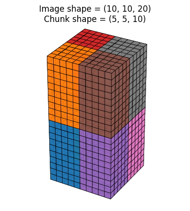
Or we could choose a smaller chunk shape:
Source
color_chunk_figure(image_shape=(10, 10, 20), chunk_shape=(2, 2, 3))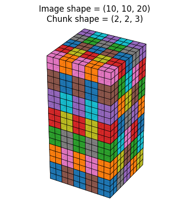
Note that the chunk shape doesn’t have to exactly divide the image shape - in the case where it doesn’t, some of the chunks on the edge are just slightly smaller than the full sized chunks.
Now if we want to load the same 8 pixels of data as before we need to load 8 chunks, but in total these contain far fewer pixels to read than when we saved the image as 2D slices. The number of pixels read are 96, versus the previous 200:
Source
fig = plt.figure()
ax = fig.add_subplot(projection='3d')

x, y, z = np.indices((10, 10, 20))

voxels = np.ones(x.shape)
voxels_request = (x < 4) & (x >= 2) & (y < 5) & (y >= 3) & (z < 4) & (z >= 2)
voxels_read = (x < 6) & (x >= 2) & (y < 6) & (y >= 2) & (z < 6) & (z >= 0)

all_vox = ax.voxels(voxels, alpha=0.2, edgecolors='black', linewidths=0.05, shade=False)
req_vox = ax.voxels(voxels_request, edgecolors='black', linewidths=0.5, facecolors='tab:red', alpha=1, shade=False);
read_vox = ax.voxels(voxels_read, edgecolors='black', linewidths=0.5, facecolors='tab:orange', alpha=0.3, shade=False);

ax.axis('off')
ax.set_aspect('equal')

custom_lines = [
    list(all_vox.values())[0],
    list(req_vox.values())[0],
    list(read_vox.values())[0]]
ax.legend(custom_lines, [
    'All data',
    f'Requested data ({np.sum(voxels_request)} voxels)',
    f'Read data ({np.sum(voxels_read)} voxels)'])
ax.set_title("Chunk shape = (2, 2, 3)")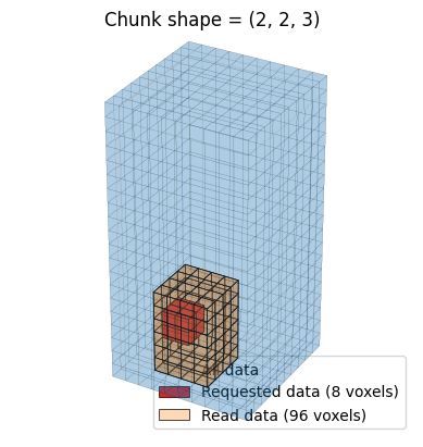
Much easier and quicker to load! In Chapter 2 we’ll see how to create a Zarr dataset, and see how the actual files are laid out when they’re saved.
Zarr is a file format that can be used to store 3D imaging data that breaks down the image into (configurably sized) chunks. Each chunk is saved to it’s own file, reducing the amount of data reading needed when only viewing a small portion of the image.
OME-Zarr
We’ve seen how Zarr solves the problem of viewing zoomed in high-resolution fields of view of our image. But what about viewing zoomed out views of the whole dataset? In this case loading the full resolution data would be wasteful because the data shape is larger than the screen that it’s being viewed on. As an example, the laptop I’m writing this on has a resolution of 2560 x 1664 and the full resolution shape of an typical dataset from the Human Organ Atlas is 7000 x 7000.
OME-Zarr solves this by providing a data format that stores both the original full resolution image as a Zarr array, and successively downsampled versions of the same dataset alongside as other Zarr arrays. This is called a multiscale image.
Source
fig = plt.figure()
original_res = np.array([10, 10, 20])
for i in range(3):
    ax = fig.add_subplot(1, 3, i+1, projection='3d')

    bin_factor = 2**i
    x, y, z = np.indices(np.ceil(original_res / bin_factor).astype(int).tolist())
    voxels = np.ones(x.shape)
    all_vox = ax.voxels(voxels, alpha=1, edgecolors='black', linewidths=1, shade=False)
    ax.axis('off')
    ax.set_aspect('equal')
    ax.set_title(f"Bin-by-{bin_factor}")

fig.suptitle("OME-Zarr multiscale image arrays")
fig.tight_layout()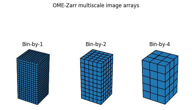
Using a multiscale image means that if you’re viewing the whole zoomed out image you can load a smaller low resolution copy of the image. As you zoom in, data from the higher resolutions is successively loaded. If you’re familiar with Google maps it works on a similar principle - as you zoom in, more detail is loaded in the location you’re viewing.
Conclusion
In this chapter we’ve seen the differences between different image compression options (lossless and lossy), and explored how the Zarr and OME-Zarr data formats can be used to store large 3D imaging data. In the next chapter, we’ll step through some practical examples of creating Zarr and OME-Zarr datasets.
For a more in-depth discussion of files, file formats, and data compression, see Chapter 6 of “Introduction to Bioimage Analysis”.